How Did the Tanh Activation Function Come Into Existence?

Have you ever wondered why tanh came into existence when we already had other perfectly logical activation functions like Sigmoid and Softmax?

Well, that’s the story we are going to uncover today. It’s a fascinating journey of solving a massive mathematical roadblock, only to run face-first into another one.

The Problem With Early Functions: The “Positive-Only” Trap

In the early days of neural networks, the Sigmoid function was the gold standard. It was logically pleasing because it squished any input into a neat range between 0 and 1, which perfectly mimics probability (like being 0% or 100% sure a picture is a cat).

The mathematical equation is elegant:

σ(x) = 1 / (1 + e⁻ˣ)

But when researchers tried to train networks with it, they hit a wall. Because Sigmoid only outputs positive numbers, the inputs passed to the next layer of the network were always positive. This created a devastating mathematical traffic jam called the zig-zag problem.

The Two-Weight Lockstep

To understand the traffic jam, let’s look at a single neuron with two incoming connections: Weight 1 (w₁) and Weight 2 (w₂). These weights receive inputs x₁ and x₂ from the previous layer.

When the network makes a mistake, it uses calculus (backpropagation) to figure out how to adjust those weights. It calculates a “Shared Error Signal” (δ) for that specific neuron. The formulas to update the weights look like this:

🔹 Update for w₁ = δ · x₁

🔹 Update for w₂ = δ · x₂

Here is the fatal flaw: If the previous layer used Sigmoid, x₁ and x₂ are always positive numbers.

Because x₁ and x₂ are both positive, and the Shared Error Signal (δ) is the exact same signed number in both equations, the updates for w₁ and w₂ are mathematically forced to have the exact same sign. If the network ideally needed to turn Weight 1 up and turn Weight 2 down to get the right answer, it literally couldn’t do it in one step. It was forced to decrease both, then increase both, over and over in a frustrating, slow zig-zag path toward the solution.

Yann LeCun’s Answer: How tanh Fixed the Flow

In 1998, AI pioneer Yann LeCun published a famous paper called Efficient Backprop. His answer to the zig-zag traffic jam was brilliantly simple: use an activation function centered around zero.

Instead of inventing new math, researchers turned to the hyperbolic tangent (tanh). The equation is essentially a shifted and stretched version of the sigmoid curve:

tanh(x) = (eˣ – e⁻ˣ) / (eˣ + e⁻ˣ)

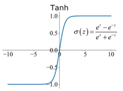
The absolute magic of tanh is its range. Instead of squishing numbers between 0 and 1, it squishes them between -1 and 1.

By simply dipping below zero, tanh shattered the lockstep problem. Now, x₁ could be a positive number and x₂ could be a negative number. Looking back at our formulas, this meant δ · x₁ and δ · x₂ could finally have opposite signs.

The network could instantly turn Weight 1 up and Weight 2 down at the exact same time, completely destroying the slow zig-zag path!

The Hidden Flaw: The Vanishing Gradient Derivation

So, did tanh solve backpropagation entirely? Unfortunately, no. While it fixed the directionality problem, tanh fell victim to an equally deadly trap when used in very deep networks: The Vanishing Gradient.

To understand why, we have to look at the derivative of tanh. The derivative (f'(z)) tells the network the slope of the curve, which is the signal it uses to learn.

Through calculus, the derivative of tanh simplifies into this beautiful trick:

f'(z) = 1 – tanh²(z)

(In plain English: 1 minus the square of the output).

But there is a fatal flaw at the edges of the curve. At the far left and far right, the tanh curve flattens out completely. If a neuron receives a large positive input (like 10), tanh squishes it to almost exactly 1. Let’s plug that output of 1 into our derivative math:

f'(z) = 1 – (1)² = 0

The slope is exactly zero.

During backpropagation, the network passes the learning signal backward by multiplying the gradients of each layer together. If a neuron is sitting in that flat region, its derivative is 0. When you multiply the incoming learning signal by 0, the signal is instantly destroyed. It vanishes.

In deep networks, multiplying these tiny fractions meant the error signal completely died before it reached the early layers. The network simply stopped learning.

The Real Savior: Enter ReLU

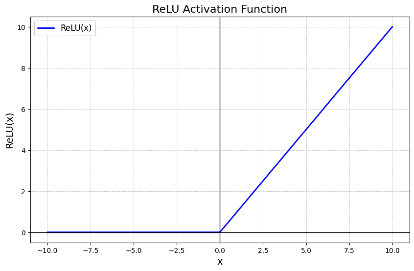
Because tanh pinched off the learning signal at its flat edges, the AI community needed a function that never flattens out on the positive side.

Enter the Rectified Linear Unit (ReLU).

The math is brutally simple:

f(z) = max(0, z)

(If the input is negative, output 0. If positive, output the number as-is).

Because a positive number just draws a perfectly straight line, its slope (derivative) is always exactly 1. It doesn’t matter if the input is 5 or 5,000. During backpropagation, the error signal can multiply by 1 through a hundred layers without ever vanishing!

Today, tanh is mostly retired from the deep, hidden layers of standard networks, making way for ReLU. However, it survives as an absolute necessity in memory-based networks (like LSTMs) where the AI needs that -1 to 1 squeezing effect to carefully control and overwrite internal memory.