Key Concepts
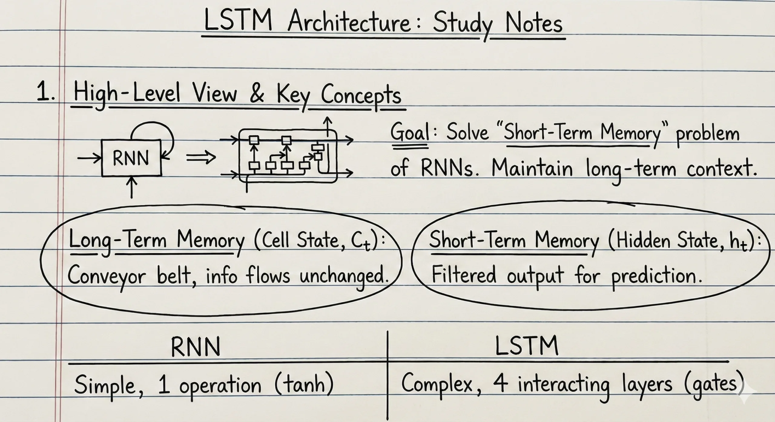
- Cell State (Ct): The long-term memory vector that flows through the network, maintaining context across time steps
- Hidden State (Ht): The short-term memory vector that serves as output for the current time step
- Forget Gate (ft): Decides what information to remove from cell state using sigmoid activation (0 = forget, 1 = keep)
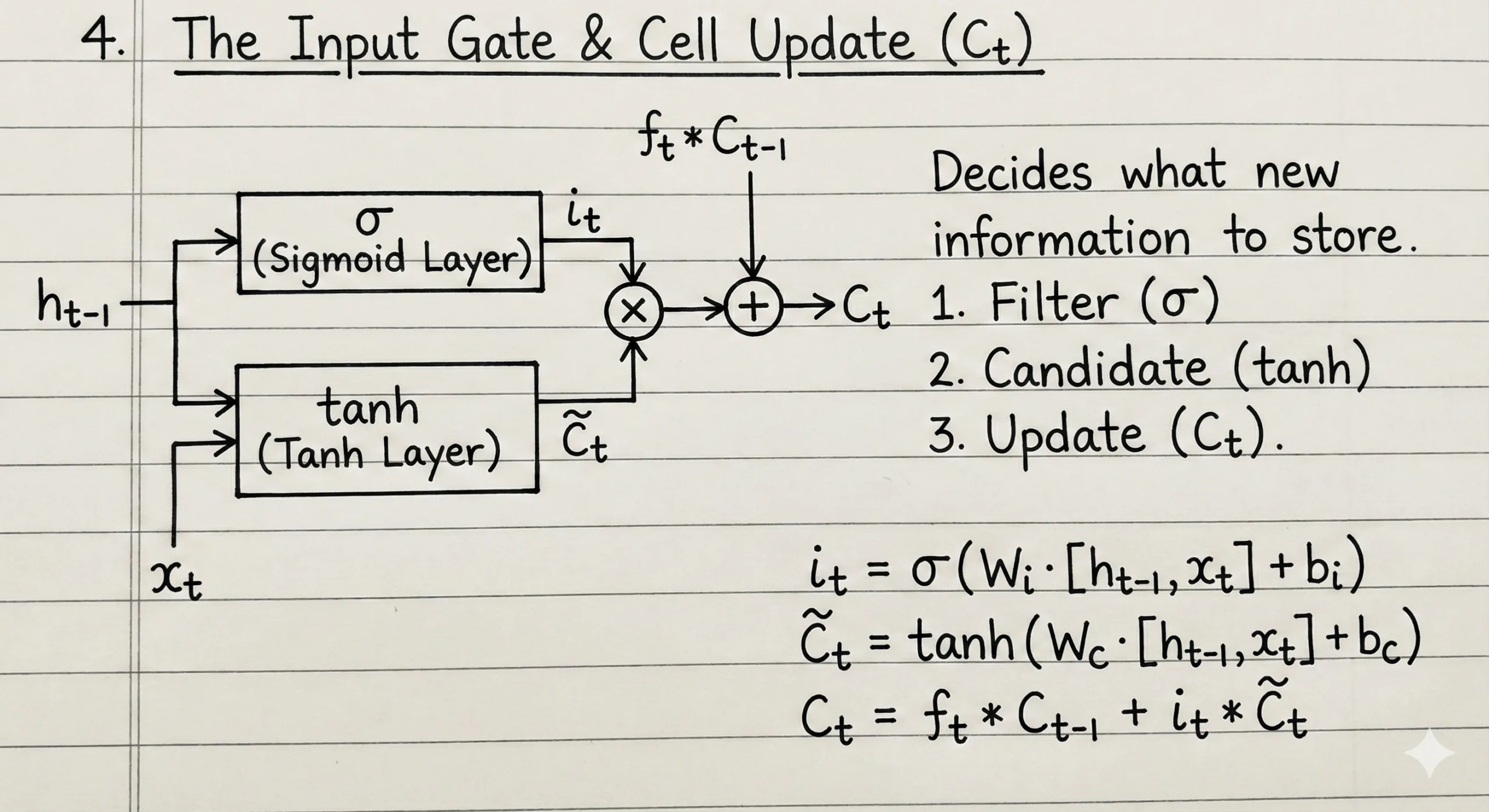
- Input Gate (it): Filters which new candidate values should be added to cell state
- Candidate Cell State (C̃t): Potential new information to add, computed using tanh activation
- Output Gate (ot): Controls what information from cell state becomes the hidden state output
- Pointwise Operations: Element-wise multiplication (⊙) and addition (+) between vectors of same dimensions
- Gate Mechanism: All gates use sigmoid activation (σ) to produce values between 0 and 1, acting as filters
What is LSTM?

Long Short-Term Memory (LSTM) is a specialized type of Recurrent Neural Network (RNN) architecture designed to solve the vanishing gradient problem and maintain long-term dependencies in sequential data. Unlike standard RNNs that struggle to retain information over many time steps, LSTMs use a sophisticated gating mechanism to selectively remember or forget information.
The fundamental innovation of LSTMs lies in their dual-memory system: a cell state (Ct) for long-term context and a hidden state (Ht) for short-term processing. This architecture enables LSTMs to excel at tasks like language modeling, machine translation, time series prediction, and sentiment analysis.
The LSTM Cell: Inputs and Outputs

An LSTM cell at time step t receives three inputs and produces two outputs:
Inputs:
Ct-1: Previous cell state (long-term memory from previous time step)Ht-1: Previous hidden state (short-term memory from previous time step)Xt: Current input (e.g., word embedding vector at current time step)
Outputs:
Ct: Updated cell state (flows to next time step)Ht: Current hidden state (used as output and flows to next time step)
All vectors maintain consistent dimensions throughout. If Ct is a 3-dimensional vector, then Ht, ft, it, ot, and C̃t will all be 3-dimensional vectors as well. This dimensional consistency is a fundamental rule in LSTM architecture.
How LSTM Works: The Gate Mechanism
Think of an LSTM like a content editor reviewing a story chapter by chapter. At each chapter (time step), the editor must decide:
- What to forget: Remove outdated plot points that are no longer relevant
- What to remember: Add new important information to the ongoing narrative
- What to output: Decide which parts of the story context to use for current understanding
LSTM accomplishes this through three specialized neural network layers called gates, each controlling information flow through filtering operations.
The entire process happens in two major steps:
- Cell State Update: Modify long-term memory by removing unnecessary information and adding new relevant information
- Hidden State Calculation: Generate short-term output based on updated cell state
Step 1: The Forget Gate

The forget gate decides what information to discard from the cell state. It’s the first gate in the LSTM processing pipeline.
Architecture:
The forget gate is a neural network layer with sigmoid activation function. It takes two inputs:
Ht-1: Previous hidden stateXt: Current input
Mathematical Operation:
ft = σ(Wf · [Ht-1, Xt] + bf)
Where:
Wf: Weight matrix for forget gatebf: Bias vector for forget gate[Ht-1, Xt]: Concatenation of previous hidden state and current inputσ: Sigmoid activation function (outputs values between 0 and 1)
How Filtering Works:
The forget gate output ft is then multiplied element-wise with the previous cell state:
Ct-1 ⊙ ft
Example: If Ct-1 = [4, 5, 6] and ft = [0.5, 0.5, 0.5], then Ct-1 ⊙ ft = [2, 2.5, 3] (50% information retained). If ft = [0, 0, 0], all information is forgotten. If ft = [1, 1, 1], all information passes through unchanged.
Step 2: The Input Gate (Adding New Information)

The input gate determines what new information should be added to the cell state. This is a two-part process:
Part A: Create Candidate Values
First, generate potential new information using tanh activation:
C̃t = tanh(Wc · [Ht-1, Xt] + bc)
The tanh activation produces values between -1 and 1, representing candidate information that could be added to cell state.
Part B: Filter Candidate Values
Next, decide which candidates are worth adding using a sigmoid gate:
it = σ(Wi · [Ht-1, Xt] + bi)
The input gate it acts as a filter, producing values between 0 and 1.
Combining Both Parts:
Multiply the candidate values with the input gate filter:
Filtered candidates = it ⊙ C̃t
Example: If C̃t = [0.8, 0.9, 0.7] (candidate values) and it = [1.0, 0.5, 0.0] (filter), then filtered candidates = [0.8, 0.45, 0]. This means:
- First value: 100% of candidate is added
- Second value: 50% of candidate is added
- Third value: Candidate is rejected (0% added)
Step 3: Updating the Cell State
Now we combine the results from forget gate and input gate to update the cell state:
Ct = (ft ⊙ Ct-1) + (it ⊙ C̃t)
This equation has two components:
ft ⊙ Ct-1: Information retained from previous cell state (after forgetting)it ⊙ C̃t: New filtered information being added
The Beauty of This Design:
Notice that this is a simple addition operation, not a multiplication through multiple layers. This is the key to solving the vanishing gradient problem in traditional RNNs. The gradient can flow backward through this additive path without diminishing exponentially.
Example:
- Previous cell state:
Ct-1 = [4, 5, 6] - Forget gate removes 50%:
ft ⊙ Ct-1 = [2, 2.5, 3] - Input gate adds new info:
it ⊙ C̃t = [0.8, 0.45, 0] - Updated cell state:
Ct = [2.8, 2.95, 3]
The LSTM has successfully updated its long-term memory by partially forgetting old information and selectively adding new information.
Step 4: The Output Gate

The final step is generating the hidden state Ht, which serves as the output for the current time step. The output gate controls what information from the cell state should be exposed.
Process:
First, apply tanh to the updated cell state to normalize values between -1 and 1:
tanh(Ct)
Then, create an output filter using sigmoid activation:
ot = σ(Wo · [Ht-1, Xt] + bo)
Finally, multiply them element-wise to produce the hidden state:
Ht = ot ⊙ tanh(Ct)
Why This Matters:
The output gate allows the LSTM to selectively reveal information from its long-term memory based on current context. Not all information in cell state needs to be exposed at every time step.
Example: If tanh(Ct) = [0.9, 0.8, 0.7] and ot = [1.0, 0.0, 0.5], then Ht = [0.9, 0, 0.35]. The output gate has chosen to expose the first dimension fully, hide the second dimension completely, and partially reveal the third dimension.
Mathematical Notation Summary
Here are the complete LSTM equations in order:
1. Forget Gate:
ft = σ(Wf · [Ht-1, Xt] + bf)
2. Input Gate:
it = σ(Wi · [Ht-1, Xt] + bi)
3. Candidate Cell State:
C̃t = tanh(Wc · [Ht-1, Xt] + bc)
4. Cell State Update:
Ct = (ft ⊙ Ct-1) + (it ⊙ C̃t)
5. Output Gate:
ot = σ(Wo · [Ht-1, Xt] + bo)
6. Hidden State:
Ht = ot ⊙ tanh(Ct)
Dimensions: If we have n hidden units (nodes) in each gate, then:
- All state vectors (Ct, Ht, ft, it, ot, C̃t) are
n × 1 - If input dimension is
m, then concatenation[Ht-1, Xt]is(n+m) × 1 - Weight matrices are
n × (n+m) - Bias vectors are
n × 1
Pointwise Operations Explained
LSTM architecture heavily relies on two pointwise (element-wise) operations:
Pointwise Multiplication (⊙):
Multiply corresponding elements of two vectors:
[a, b, c] ⊙ [x, y, z] = [a×x, b×y, c×z]
Example: [4, 5, 6] ⊙ [0.5, 0.5, 0.5] = [2, 2.5, 3]
Pointwise Addition (+):
Add corresponding elements of two vectors:
[a, b, c] + [x, y, z] = [a+x, b+y, c+z]
Example: [2, 2.5, 3] + [0.8, 0.45, 0] = [2.8, 2.95, 3]
These operations are computationally efficient and preserve vector dimensions, making them ideal for controlling information flow in neural networks.
Why Sigmoid and Tanh?
Sigmoid (σ) for Gates:
Sigmoid outputs values between 0 and 1, making it perfect for filtering:
σ(x) ≈ 0: Block information completelyσ(x) ≈ 0.5: Let 50% of information throughσ(x) ≈ 1: Let all information pass through
This is why all three gates (forget, input, output) use sigmoid activation.
Tanh for Values:
Tanh outputs values between -1 and 1, allowing the network to:
- Represent both positive and negative updates
- Center the data around zero for better gradient flow
- Provide stronger gradients than sigmoid in the middle range
This is why candidate cell state and the final cell state transformation use tanh.
LSTM vs Standard RNN
Standard RNN Problem:
In vanilla RNNs, hidden state is updated via:
Ht = tanh(W · [Ht-1, Xt] + b)
During backpropagation through many time steps, gradients are multiplied repeatedly by weight matrices, causing them to either vanish (→0) or explode (→∞). This makes learning long-term dependencies nearly impossible.
LSTM Solution:
The cell state update equation:
Ct = (ft ⊙ Ct-1) + (it ⊙ C̃t)
Uses addition instead of multiplication, creating a “gradient highway” that allows gradients to flow backward without vanishing. When ft ≈ 1 and it ≈ 0, information from Ct-1 passes almost unchanged to Ct, preserving long-term dependencies across hundreds of time steps.
This architectural innovation is why LSTMs can successfully model dependencies in long sequences where RNNs fail.
Practical Implementation Considerations
Choosing Hidden Units:
The number of hidden units (dimension of Ct and Ht) is a hyperparameter you must set:
- Small datasets: 64-128 units
- Medium datasets: 128-256 units
- Large datasets: 256-512 units
- Very large datasets: 512-1024 units
Weight Initialization:
Forget gate biases are often initialized to positive values (e.g., 1.0) to encourage remembering information initially, allowing the network to learn what to forget during training.
Computational Cost:
LSTMs have 4× more parameters than vanilla RNNs (three gates + candidate cell state, each with their own weights). This means:
- Longer training time
- Higher memory requirements
- Better performance on complex sequential tasks
Common Applications:
- Machine translation (encoder-decoder architectures)
- Text generation and language modeling
- Speech recognition
- Time series forecasting
- Video analysis and action recognition
- Sentiment analysis on long documents
Variants and Extensions
GRU (Gated Recurrent Unit):
A simplified version of LSTM with only two gates (reset and update), fewer parameters, and faster training. Often performs comparably to LSTM on many tasks.
Bidirectional LSTM:
Processes sequences in both forward and backward directions, capturing context from both past and future. Useful when entire sequence is available (not for real-time prediction).
Peephole Connections:
Modified LSTM where gates can “peek” at the cell state directly:
ft = σ(Wf · [Ct-1, Ht-1, Xt] + bf)
This gives gates more information for decision-making but adds complexity.
Stacked LSTMs:
Multiple LSTM layers stacked vertically, where the hidden state output of one layer becomes the input sequence for the next layer. Increases model capacity for complex patterns.
Conclusion
LSTM architecture elegantly solves the long-term dependency problem through its gating mechanism and additive cell state updates. By understanding each gate’s role—forget gate for removing irrelevant information, input gate for adding new information, and output gate for controlling what to expose—you can appreciate why LSTMs became the standard for sequential modeling tasks.
The key insight is that LSTMs don’t just process sequences; they intelligently curate information flow through learned filtering operations. Each gate is a trainable neural network layer that learns what to remember, what to forget, and what to output based on the task at hand.
While modern architectures like Transformers have surpassed LSTMs in many NLP tasks, LSTMs remain relevant for time series analysis, real-time sequence processing, and scenarios with limited computational resources. Understanding LSTM architecture provides foundational knowledge for grasping more advanced sequence modeling techniques.
Discover more from WireUnwired Research
Subscribe to get the latest posts sent to your email.


